Rod Hyman Expert Valuer

Estimating deterioration and physical obsolescence of plant and equipment using a modified age/life formula.

 

The art of keeping it simple, but not simpler

 

By Alexander Lopatnikov, ASA and Rodney Hyman, LFAPI FRICS ASA

 

The wider adoption of fair value accounting in recent years drawn significant attention to valuation issues. In the aftermath of the global financial crisis, the priority of developing robust valuations of financial instruments is unsurprising. At the same time, various issues in the valuation of plant and equipment assets remain unresolved.

Being principles-based, financial reporting standards are not prescriptive with respect to the ways valuations of assets are to be performed. However, financial reporting practices inevitably impact thinking and logic embodied in the International Valuation Standards and its application by valuation practitioners.

This paper discusses prevailing practices of estimating physical deterioration (or physical obsolescence, terminology introduced in the latest IVS2017) of tangible assets over their useful lives. We argue that both the terminology and methodology of the most often used age/life method requires further clarification and improvement. We suggest a modified age/life formula for use in the valuation of plant and equipment of asset-heavy companies.

Valuation of plant and equipment assets includes an analysis of their utility consumption or a decline in resale price with age or use. Professional valuation standards differentiate the concepts of price and value, which does not preclude price to be a measure of value (however price does not always represent value). Moreover, the financial reporting standards claim that the exit price is the proper measure of an asset’s fair value. One could argue that plant and equipment assets are unlikely bought for resale (except as inventory) prior to the expiration of their useful lives (which is in a way similar to financial assets held to maturity). The exit price of an individual piece of equipment may rather be a measure of the asset’s orderly liquidation value, not its market value in continued use. What is even more important for the purpose of this article - measuring value as the price in the secondary market is not possible for the specialized plant and machinery, which by definition is rarely if ever, sold in the market, other than part of the business it is used in.

In those cases where assets, similar to some elements of specialized plant and equipment are bought and sold in the secondary market, one should carefully analyze if prices of those transactions are indeed indicative of the value for the assets. The use of generally lower prices (due to information asymmetry or other market peculiarities) reported in the secondary market transaction with selected equipment part of a larger specialized unit that does not evidence economic obsolescence, may effectively result in a transfer of value to other assets or goodwill. Further, many of the users of these specialised assets are by nature unlikely to ever purchase these assets unless new and then only from an OEM.

If market price (exit price) is not the right measure of the decline in value of the specialized plant and equipment, what is? In practice, this diminution of value is estimated during appraisal, with consideration of all forms of deterioration and obsolescence, and using certain formulas and professional judgment.

IVS 2017 defines items of plant and equipment (also known in the English-speaking countries as personal property) as “tangible assets that are usually held by an entity for use in the manufacturing/production or supply of goods or services, for rental by others or for administrative purposes and that are expected to be used over a period of time.”

The period of use is called useful life, with the definition adopted from IFRS - Useful Life (IFRS Definition from IAS 16): (a) the period over which an asset is expected to be available for use by an entity; or (b) the number of production or similar units expected to be obtained from the asset by an entity. Perhaps the author should have added the words “when new”. 

Definitions from various ASA sources  Useful life: The period of time over which property may reasonably be expected to perform the function for which it was designed. Normal useful life (NUL): The estimated number of years that a new property will actually be used before it is retired from service. Physical life (Normal Useful (Physical) Life, NUL): The number of years that a new property will physically endure before it deteriorates or fatigues to an unusable condition, purely from physical causes without considering the possibility of earlier retirement due to functional or economic obsolescence. (It is derived from mortality data and the study of specific assets under actual operating conditions.) Economic life: The estimated number of years that a new property may be profitably used for the purpose for which it was intended. (This time span may be limited by changing factors of obsolescence and physical age.) Remaining useful life: The estimated period during which a property of a certain effective age is expected to actually be used before it is retired from service. Remaining economic life: The estimated period during which a property of a certain age is expected to continue to be profitably used for the purpose for which it was intended Effective age: The apparent age of an asset in comparison with a new asset of like kind (That is the age indicated by the actual condition of a property). Residual value: For a tangible asset, the term that refers to the value of an asset after expiration of its normal useful life Residual value (accounting): The estimated net scrap, salvage, or trade-in value of a tangible asset at the estimated date of disposal; also called salvage value or disposal value

 
IVS also defines economic life, as “the total period of time over which an asset is expected to generate economic benefits for one or more users.”¹

The IVS glossary does not specifically define physical life, but IVS 300 provides the following description in para 80.3. related to the analysis of Depreciation and Obsolescence “The physical life is how long the asset could be used before it would be worn out or beyond economic repair, assuming routine maintenance but disregarding any potential for refurbishment or reconstruction.”. On the first reading the above looks clear although it omits the word “entity” or “user”. This is a significant issue as the asset with a life of n years in one application may have a life of n+ years in another. In practice, however, what constitutes routine maintenance and what does not is a matter of judgment. Oftentimes companies in the same industry are not consistent in the way they capitalize repairs and overhauls and oftentimes the distinction is tax driven rather than “valuation”.

The same IVS 300 paragraph expands and further clarifies the definition of economic life as follows: “The economic life is how long it is anticipated that the asset could generate financial returns or provide a non-financial benefit in its current use. It will be influenced by the degree of functional or economic obsolescence to which the asset is exposed.” We would like to stress that, according to the standard, the benefits over the economic life of an asset can be both financial and non-financial. Unfortunately, the standard does not go further to explain if it means absolute or relative financial benefits (a machine can be useful, but marginally profitable, i.e. not earning a return that a modern replacement machine would generate or in that particular application earning a return that would be insufficient against the capital cost of a replacement machine).

American Society of Appraisers ME201 Introduction to Machinery and Equipment Valuation provides a generally similar, and broader set of definitions, introducing normal useful life, remaining lives and residual values. The ASA definitions are also not specific on what kind of profitability should be considered. The concept of effective age is added for the use in calculations of physical deterioration or obsolescence.

The Uniform Standards of Professonal Appraisal Practice published by the Appraisal Foundation (2016-17 Edn) (USPAP) also introduces the terms “effective age and remaining life²“ “economic life³” and “remaining economic life⁴”.

Value of plant and equipment assets declines as they age due to wear and tear and various forms of obsolescence, the process usually called depreciation. A recent guidance note produced by RICS⁵ stresses the importance to understand that the word ‘depreciation’ is used in a different context for valuation than in financial reporting. “In valuation, ‘depreciation’ refers to the reduction, or writing down, of the cost of a modern equivalent asset to reflect the subject asset’s physical condition and utility together with obsolescence and relative disabilities affecting the actual asset. In financial reporting, ‘accounting depreciation’ refers to a charge made against an entity’s income to reflect the consumption of an asset over a particular accounting period.”

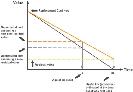
This article only addresses physical deterioration of plant and machinery. An illustration of the value decline over the useful life of a plant and machinery asset due to various factors is provided in the following picture.

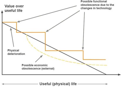
It is important to remember that the loss in value over the life of the asset is not necessarily linear or occurs in equal portions over equal periods of time. The latter are usually selected to be equal to accounting periods, and one year may not necessarily represent typical use or maintenance period. Furthermore, the value may reverse as illustrated below.

• the value of machinery will depend not only on its age, but a certain use parameter, say working hours of an engine, or hydraulic system. Similar assets with equal age may be used up differently, hence resulting in different values.
• many machinery assets are manufactured in countries or economic zones different to the one in which the machinery is found. Exchange rate movements can have a big impact on current replacement cost against historical cost. By example in 2009 the Australian dollar purchased just US65c. In 2011 it purchased for a short time more than $1.10 and stayed at more than 95c for almost 2 years. During this period any valuer applying the cost approach was likely to have found that many machinery assets in Australia increased in value.
• post the financial crisis in 2008, mobile drill rig manufacturers could not keep up with demand. Used drill rigs commanded a premium to the extent that anyone with an order close to fulfillment could sell their place in the queue quite easily and any second-hand drill rig in reasonable condition and less than say 5 years old could be sold for or close to new replacement cost. Similar situation may occasionally occur in cyclical industries, like steel and metals.

Para 80.4 and 80.5 of IVS 300⁶ provide a recommendation on how the decline in value could be measured.

Except for some types of economic or external obsolescence, most types of obsolescence are measured by making comparisons between the subject asset and the hypothetical asset on which the estimated replacement or reproduction cost is based. However, when market evidence of the effect of obsolescence on value is available, that evidence should be considered.

Physical obsolescence can be measured in two different ways:
(a) curable physical obsolescence, ie, the cost to fix/cure the obsolescence, or
(b) incurable physical obsolescence which considers the asset’s age, expected total and remaining life where the adjustment for physical obsolescence is equivalent to the proportion of the expected total life consumed. Total expected life may be expressed in any reasonable way, including expected life in years, mileage, units produced, etc.

The above suggests the use of age/life method for estimating incurable physical obsolescence. The following factors are recommended to normally be considered in the valuation of plant and equipment with suggested amendments by these authors (noted in square brackets:

1. the asset’s technical specification,
2. the remaining useful, economic or effective life [to the entity], considering both preventive and predictive maintenance,
3. the asset’s condition, including maintenance history,
4. any functional, physical and technological obsolescence,
5. if the asset is not valued in its current location, the costs of decommissioning and removal, and any costs associated with the asset’s existing in-place location, such as installation and re-commissioning of assets to its optimum status,
6. for machinery and equipment that are used for rental purposes, the lease renewal options and other end-of-lease possibilities,
7. any potential loss of a complementary asset, eg, the operational life of a machine may be curtailed by the length of lease on the building in which it is located [or the remaining availability of a resource required for its continued operation],
8. additional costs associated with additional equipment, transport, installation and commissioning, etc, and
9. in cases where the historical costs are not available for the machinery and equipment that may reside within a plant during a construction, the valuer may take references from the Engineering, Procurement, Construction (“EPC") contract.

Consideration should also be given to environmental- and economic-related factors.

The definition and basics of the age/life analysis are provided in the ASA ME201 as follows.

The age/life analysis is a part of the process by which a property’s remaining useful life (and consequently its value) may be established. In the broadest sense, straight-line depreciation is generally being considered in an age/life analysis. Age/life analysis establishes the arithmetic life cycle of the assets at the effective date of the appraisal. When adjustments are required for observed conditions relating to use, physical condition, and obsolescence, this analysis may be a major tool.

The key steps in the age/life study should include the following.

1. Inspection of the subject property and determining its condition,
2. Examination of the client’s records,
3. Establishment of a normal useful life for the subject,
4. Establishing effective age or remaining useful life⁷ , and
5. Mathematically determining physical depreciation.

The description further notes that “on relatively new items having a short expired life and where little or no obsolescence has occurred, the total life, normal life, and remaining useful life are more nearly equal.”

New items provide a special challenge as we can observe market behavior for many assets which are almost new and which indicate that the expired portion of their life has a disproportionate effect on value. We are all aware that a motor vehicles loses value as it is driven out of the new car showroom. This loss in value reflects economic obsolescence so valuers should be wary of thinking that a relatively new item has only a small physical obsolescence as physically and technologically it is no different to the one still sitting in the showroom. It is factors external to the asset that determines the loss in value.

ASA ME201 explains that age/life analysis is a technique ”for measuring physical deterioration... Other techniques include observation in dollar terms or as a percentage of new. The Age/Life formula or ratio is explained to mean “chronological age divided by normal useful life.” At the same time, the formula provided to illustrate the concept refers to the effective age.

The cautionary note that one should “remember that normal useful life is established at the time an asset is put into service…” only adds to the confusion. The guidance then explains the relationship between NUL, effective age, and RUL as follows.

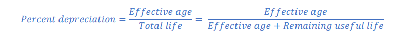
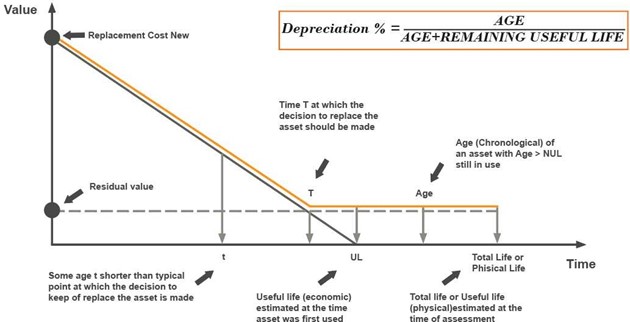
Valuers need to be aware that in the above equation the remaining useful life is usually the driver, with effective age being a derivative parameter. In addition, so-called, “normal” useful life may change over the life of the asset. Considering the above a more practical notation of the formula for percent depreciation is as follows.

The following comment provided in the MTS guidance is particularly important in practice. “Total life can include an extension of the normal life expectancy due to past use, above average maintenance, capital additions, rebuilds and upgrading, which enable the asset to remain cost-effective when compared with that representing current technology. This is usually the case when a machine that has a normal useful life of 25 years is found to be functioning even after 30 years, 40 years, 50 years, or more.” The corollary of this proposition is also true: total life can include a reduction of the normal life expectancy due to past use, below average maintenance, lack of rebuilds as required and nil or almost no upgrading in line with market practice.

Our experience is that this situation is typical for asset-intensive companies where fully depreciated assets (with net book value equal to zero) may account for 50% and more of the total number of plant and machinery assets. The number of assets fully depreciated for tax purposes is often even larger since tax depreciation differs from GAAP in three respects: (a) a mandated or preferred tax life, which is typically shorter than the economic life; (b) cost recovery on an accelerated basis, and (c) an assigned salvage value of zero. One should also recognize that many companies adopt tax value for accounting value.

 

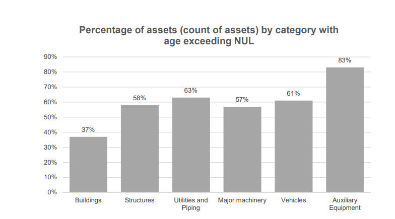
The above real-life picture illustrates the percentages of assets by category with ages exceeding their normal useful lives for an asset-heavy company. We can see that not only the share of such assets is significant, but that it is high for all asset classes. Which raises the question, how normal are those “normal” useful lives used by the companies and valuers.

IFRS (IAS 16 Property, Plant and Equipment) requires the entity to select the method that most closely reflects the expected pattern of consumption of the future economic benefits embodied in the asset. The pattern of consumption of future economic benefit, useful life, and residual value need to be reassessed at year-end, and the depreciation method adjusted if there are any significant changes.

The results of the assessment need to withstand an extensive audit process, consideration needs to be given to ensure that the auditors will be able to obtain sufficient and appropriate evidence with respect to the critical assumptions adopted within the methodology (including useful life and residual value) and that the methodology is logical and consistent with the entity’s understanding of how the asset’s service potential is consumed.

In practice, however, annual reassessment of assets remaining useful life and residual value is rare being burdensome for asset-heavy companies whose asset records include tens or even hundreds of thousands of plant and machinery entries. Moreover, auditors focus more on assets with potentially overstated carrying values, than understated plant and equipment.

The appeal of the straight-line method, i.e. it is simple and easily understood, makes it the most commonly used method of depreciation⁸. As more data about replacement patterns and consumption of plant and machinery is accumulated in corporate information systems, some entities may apply non-linear patterns of consumption. In practice, however, the majority of financial statements of companies are prepared under the assumption that the pattern of consumption for most assets is constant and therefore justifies use if the straight-line method.

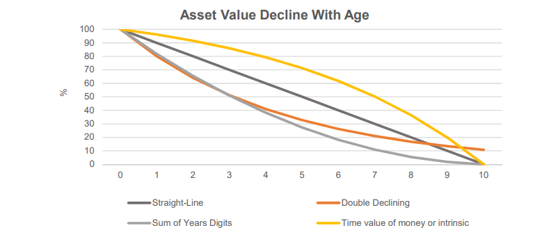
It is worth noting that accounting rules allow the use of double declining depreciation method and sum of the years’ digits methods as illustrated in the picture below⁹. If the time value of money would have been taken into account in estimating depreciation of an asset, which is not admitted anywhere in the world, the depreciation curve may have looked like the yellow line on the chart.

Some valuation practitioners advocate the use of a so-called, S-curve pattern of consumption, i.e. with a higher (or lower) rate of consumption in the early years, flattening out later and then either increasing (or decreasing) as the asset approaches the end of life.

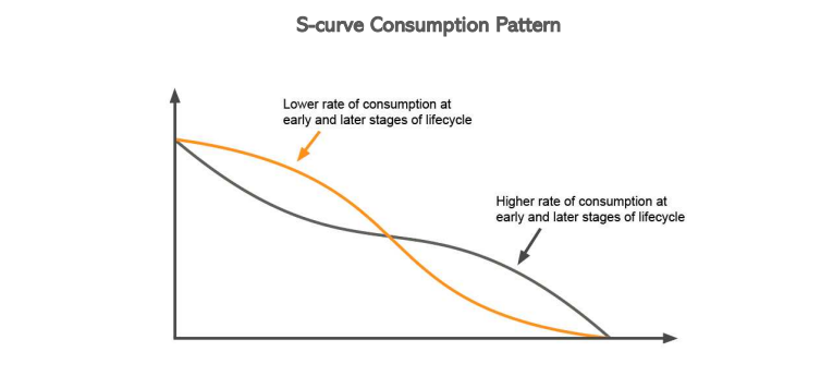
They argue that this pattern is suitable for some types of residential or commercial properties or even motor vehicles and more closely reflects the market price movements of assets commonly traded in open markets.

The use of an S-curve may be justified for valuation of some individual assets provided sufficient data is available to support the fact, that the curve represents the likely reality.¹⁰ The following two factors need to be taken into consideration when referencing research publications. The researchers analyzed price decline in the secondary market (primarily auction and dealer pricing), assuming value in exchange, not value in use of the assets. The auction prices for individual pieces of machinery may not necessarily proxy the actual cost to replace the existing fleet of equipment. Valuers are advised to carefully analyze market participants decision-making process and preferences when sourcing main equipment. Including their typical suppliers and risk factors involved in buying from the secondary market.

The picture below illustrates auction price decline profile for specialized equipment, which implies accelerated decline in the first few years of use (period “A”), followed by a longer period of relatively slow decrease in value (period “B”), and period of prices falling faster to zero or scrap value (period “C”).

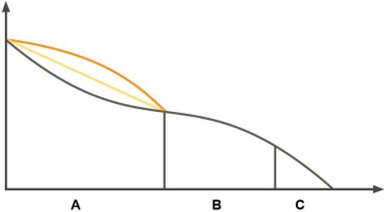
Interestingly, a review of auction data, indicates that supportive evidence for period “A” (one to three years old equipment) is usually scarce and in most cases absent, since the market for “almost new” equipment is limited, if at all exiting, other than sales in a distressed context. This makes price estimates during the period “A” highly uncertain and unreliable. A proverbial belief that a car leaving dealer’s shop loses 10 to 20% percent of its price (not necessarily value) is more a behavioral pattern (information asymmetry) hence not an indication of aging, i.e. physical deterioration.

Period “C” is also characterized by significant uncertainty with little evidence available to establish when exactly assets are «normally» discontinued, or whether the decision to replace them is a result of wear and tear, or other, mostly economic reasons. A well-known fact that in different markets replacement of assets happens at different age only complicates the picture further.

An example from a consumer market illustrates that the useful life is country specific¹¹. The statistics of smartphone holding periods varies 10-15% of the average of 21 months. Recent data reported by Apple indicates that the upgrade cycle for iPhones was around every 3 years in fiscal 2018, and about every 4 years in fiscal 2019. ¹²

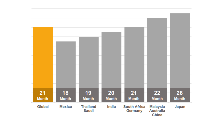
Not only the holding period is different in different countries, but reasons for why it is different may vary depending on various economic, regulatory and behavioral factors.

The typically used sources for normal useful life are provided below.

• Dealers or manufacturers of new and used equipment
• Engineering studies/firms • Articles on various industries/equipment
• Engineers of the company that owns the assets
• American Society of Appraisers NUL study
• Marshall Valuation Services
• Specialty guides
• The Iowa Curves
• The entity’s own asset register

Valuers can use their own estimates, so long as those are explained and supported. Normal lives for long-lived specialized assets¹³ are particularly difficult to estimate and these assets usually account for most of plant and machinery of asset-heavy companies.

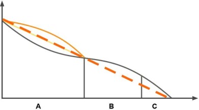
Taking the above in consideration use of a straight-line as illustrated in the picture above) may be a reasonable approximation for the decline in value of a fleet of specialized plant and equipment, specifically when valued assuming continued use.

ME201 does not explicitly mention the residual value in their age/life method examples. At the same time, a basic formula used for depreciation in any accounting book includes residual value.

Despite a general straight-line formula includes residual value, accountants prefer the use of a simplified version of it with the residual values equal to zero. This reflects a high level of uncertainty about residual value particularly if any value can at all be realized when the asset stops operating. Companies also want to make sure investment cost has been fully depreciated. As we previously noted, tax depreciation calculations do not take residual value into account.

This reasonable simplification, however, results in an inconsistency due to the fact that most companies do not regularly check useful lives of the assets while keeping them in operation longer, and oftentimes much longer than their normal useful lives.

As a result, companies’ asset registries report many totally depreciated assets, e.g. with book values equal to zero. When the fair value of these assets is assessed in a valuation, say as part of a purchase price allocation exercise or when assets are valued for financing. Since assets are still in use benefiting the owner intuition says, their value should not zero. Then question what is the right way to assess depreciation due to age and wear and tear?

A picture below illustrates depreciation profiles with and without consideration of residual value.

The valuer needs to find a way to support an estimate of the residual value of the asset. The following may be considered.

• Sales of similar equipment (may not be easy to find similar equipment or adjust the sales for differences in use (installed) and in exchange premises);
• Company’s estimates of such value and usual way to dispose of the asset (scrap or sell);
• Rule of thumb
• A percent of current replacement cost assessed on the basis of what the salvageable parts of the asset would be worth in today’s money. It is generally quite possible to assess which parts of a machine will have a value at end of life.

At the time when a plant and machinery asset is commissioned an estimate of residual value is difficult to make. There is significant uncertainty associated with it. Moreover, this estimate may change over the life of the asset. Companies and their auditors usually consider the residual value of plant and machinery assets to be equal to zero unless solid evidence to the contrary exists.

Often the evidence can be deduced from whether there is a secondary market for a machine which may have reached ‘the end of life” in its primary market or even the salvageable components of the machine. By relating the present sale to current replacement cost (RV), value can be expressed as a percentage of RV. Having said this, the uncertainty about residual value arguably decreases as asset approaches the end of its useful life, still, it remains high.

Accordingly. if no break or sudden and unexpected change in the market situation occurs the business decision of reassessing the remaining useful life is made closer to the end of the asset’s useful life with consideration of the company’s replacement practices and time required to fund, engineer, order, procure, install and test the replacement.

It could, therefore, be reasonable to use the assumption of zero residual value (unless strong evidence to the contrary is available or an assessment can be made as discussed elsewhere in this paper) until such time when the reassessment is made and when the remaining life and residual value can be estimated with higher certainty.

The residual value of the plant and machinery asset may be set equal to disposal value if it can be reasonably estimated or may be estimated as a present value of expected benefit over the remaining life (assuming continued use and if such benefit can be estimated), or using some simplified formula or rule of thumb (say a percentage of the asset’s current replacement cost new).

In theory, companies should regularly reassess assets’ remaining lives. IFRS requires it to be done annually. In practice, however, most companies do not have a regular procedure or a schedule for assessing assets remaining life and decommissioning points.

When valuing plant and machinery of a large asset-heavy company, valuers cannot verify the condition, hence effective age, for most of the individual fixed assets, since there are thousands and thousands of such assets at even a relatively small plant. We suggest that valuers may consider the following:

• When the asset is approaching its useful life or had exceeded it but is still in operation and information about the company’s plans to retire the asset is not available, the assumption can be made that it will serve for at least so long as would be required to replace it, if the decision would have been made on the date of valuation.
  • For longest-lived assets, i.e. buildings, structures, and main production units a period of 3, or even 5 years may be considered, since decisions to replace such assets is made at least that much years prior of their disposal (companies need to engineer, order, procure, install and test the replacement assets before putting them into operation).
  • For smaller individual specialized equipment with a track record of being used for longer than their normal useful lives, this period may be set at 2-3 years.
  • For other equipment, where evidence exists that it serves for longer than normal life, a one-year period (typical budget period) could be used
• Often a company’s own asset register will indicate useful lives of assets in that enterprise. If a company runs say 50 identical or similar machines each with an NUL of 30 years and there are a number of machines with ages of say, 35 years, 38 years and 40 years it might be safe to assume that NUL is 38 years especially if anecdotal evidence is available that newer machines in the fleet replaced machines with similar ages.
• When valuers assess remaining useful life (RUL), they often rely on internal maintenance records, the visual condition of the assets in terms of elapsed age and information provided by engineers within the business. This may allow the valuer to determine RUL on an average per asset category. These authors believe that such an assessment will not be less reliable than using normal useful life as the criterion and likely to be significantly more reliable.

These assumptions should be supported by statistics of physical life, or use of similar assets, which helps to set an upper-bound estimate of the physical life to the asset. In most cases, it will likely be a conservative estimate.

The advantage of the proposed procedure is in that it allows for consistency with accounting depreciation over most of the life of assets and also avoids the controversy which may arise when the valuation results in a step-up of values for assets near or exceeding their normal useful lives. It is particularly useful in valuations of individual plant and equipment assets of large companies, with many thousands or even hundreds of thousands of assets.

If the age of the plant and machinery assets systematically exceeds their useful lives selected for financial reporting purposes, the company may elect to change them to reflect a more realistic consumption pattern.

Albert Einstein famously said, that “everything should be made as simple as possible, but not simpler”. This fully applies to estimates of physical deterioration and obsolescence using the age/life method. Simplicity and transparency are important for making a sound and supportable assessment of diminution of value due to age and use. At the same time valuers need to make sure they do not oversimplify and are consistent in their valuations.

---

¹ https://www.ivsc.org/standards/glossary
² Pages 20 and 42
³ Page 157
⁴ Page 327
⁵ Depreciated replacement cost method of valuation for financial reporting, RICS guidance note 1st edition, November 2018
⁶ General Standards – IVS 105 Valuation Approaches and Methods, p. 46-47
⁷ This process typically includes establishing effective age or remaining useful life by determining the remaining useful economic life of the asset and adding the expired life of the asset to determine its normal useful life in its continued use by the current entity.
⁸ Other methods of depreciation, i.e. condition and consumption-based methods, are used for specific assets and industries and may not be related to physical deterioration of the assets.
⁹ A comparison of depreciation methods applied to an asset with a replacement value of $100 and a lifetime of 10 years; specifically, Intrinsic ( r = 20%), Straight-line, Double Declining Balance and Sum of Years Digits.
¹⁰ RICS Red Book GN 6 Replacement cost method of valuation for financial reporting
¹¹ https://www.counterpointresearch.com/smartphone-users-replace-their-device-every-twenty-one-months/
¹² https://www.cnbc.com/2019/02/08/apple-iphone-replacement-cycle-slowing-toni-sacconaghi-says.html
¹³ ‘According to IVS specialized asset is an asset “that is rarely, if ever, sold in the market, except by way of a sale of the business or entity of which it is part, due to the uniqueness arising from its specialised nature and design, its configuration, size, location or otherwise.